
This visualization project concerns the $(5,5,5)$ triangle reflection group $$ \Gamma = \langle a,b,c \: | \: a^2 = b^2 = c^2 = (ab)^5 = (bc)^5 = (ca)^5 = 1 \rangle, $$ the homomorphisms from this group into the complex Lie group $\SL_3\C$, and the open subset of Anosov homomorphisms.
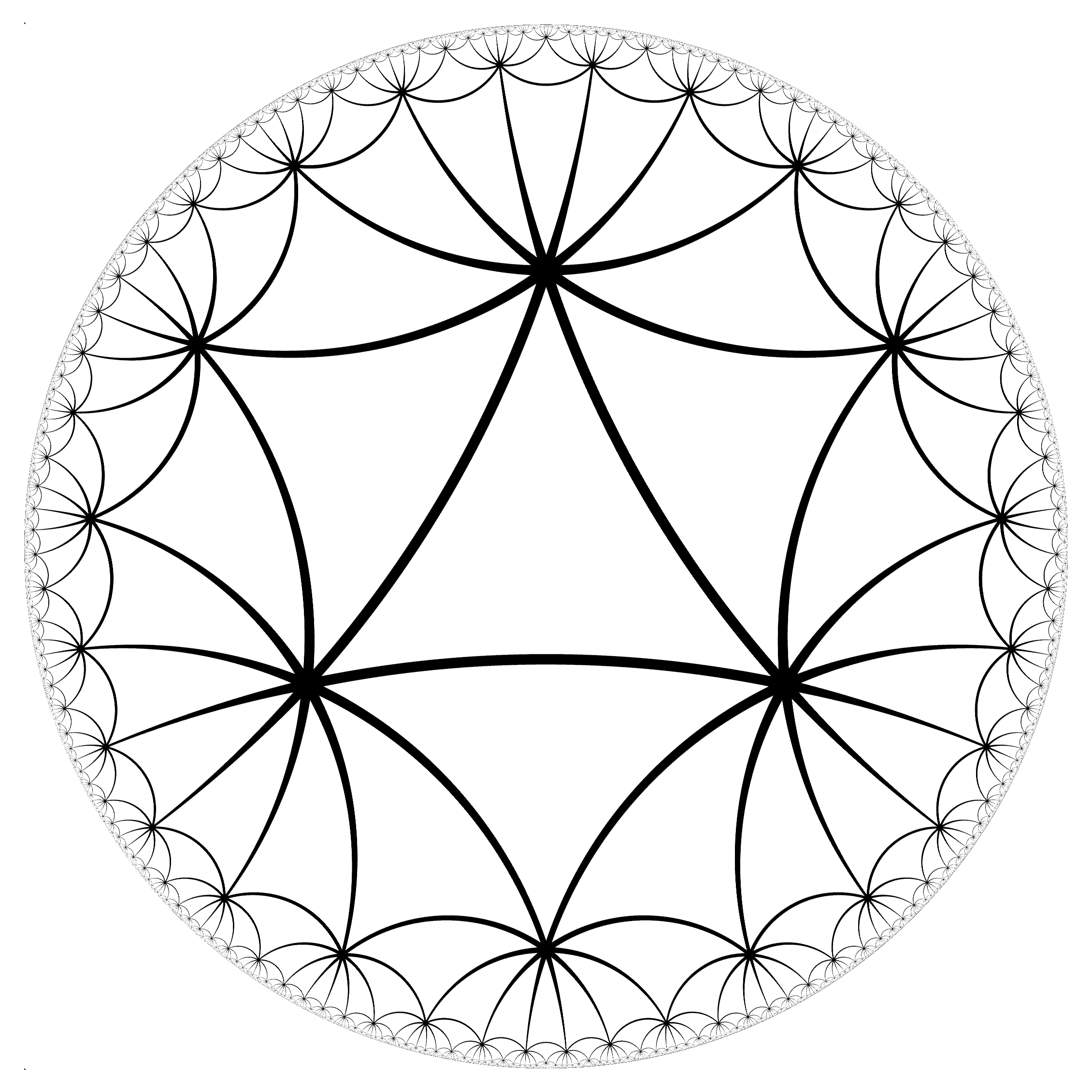
The group $\Gamma$ arises naturally as the set of isometries of the hyperbolic plane preserving the tiling by triangles shown below, and the associated embedding $\Gamma \to \Isom(\H^2)$ is rigid. This motivates the consideration of a higher-rank Lie group (as in this project) so that a nontrivial space of deformations arises.
Lee, Lee, and Stecker [1] studied homomorphisms of $\Gamma$ and other triangle groups into $\SL_3\R$, where they were able to explicitly characterize the Anosov set within the real one-dimensional space of conjugacy classes of homomorphisms. Specifically, they found the Anosov set is homeomorphic to a union of open intervals.
Passing to the complex case gives an Anosov set that lies in a complex one-dimensional deformation space, offering the possibility of a more complex shape. The aim of this project was to make computer images of the Anosov set to better understand its shape, and to formulate questions and conjectures based on the results.
There are two posters, each meant to be printed on 11x17 inch paper. The bottom section of each poster briefly summarizes what is pictured, while this document serves as a more detailed explanation. High-resolution images of the posters can be downloaded here:
These are released under a CC BY-NC 3.0 License.
Want a printed poster? You can take the high resolution images linked above to a print shop, or you can email me and ask for one (supplies limited).
Some background is needed to explain the contents of the posters.
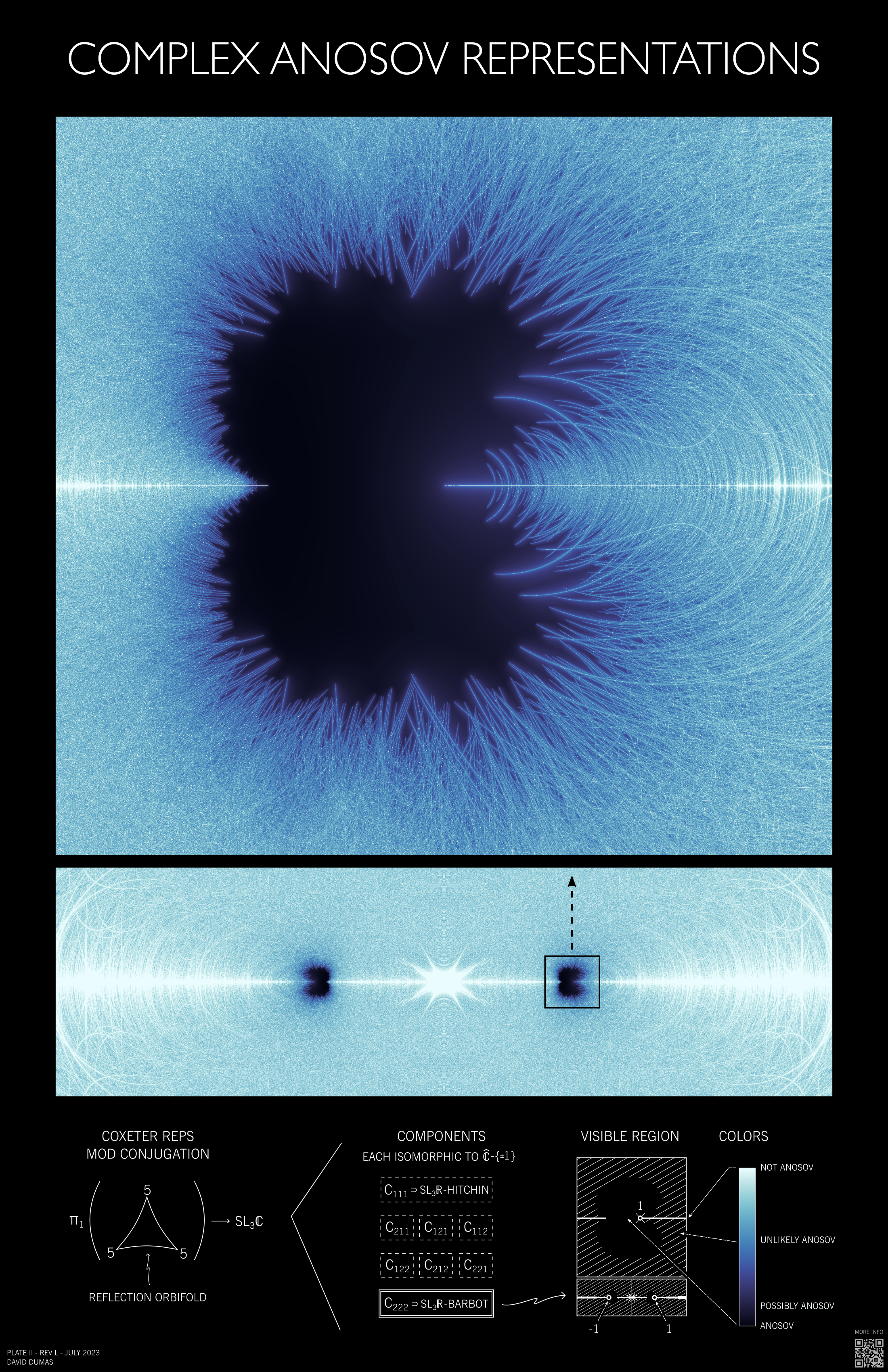
Let $\hat{\C} = \C \cup \{ \infty \}$ be the extended complex plane. For $k \in \{1,2\}$ and $s \in \hat{\C} \setminus \{ -1,1 \}$, define a homomorphism $\rho^k_s : \Gamma \to \SL_3\C$ by $$ \rho^k_s(a) = \begin{pmatrix} 1 & c_k & c_k\\ 0 & -1 & 0\\ 0 & 0 & -1\end{pmatrix}, \; \rho^k_s(b) = \begin{pmatrix} -1 & 0 & 0\\ c_k & 1 & \tau(s) \, c_k\\ 0 & 0 & -1\end{pmatrix}, \; \rho^k_s(c) = \begin{pmatrix} -1 & 0 & 0\\ 0 & -1 & 0\\ c_k & \tau(s)^{-1} \, c_k & 1\end{pmatrix} $$ where $$ \tau(s) = \frac{1+s}{1-s}, \; c_1 = \frac{-1-\sqrt{5}}{2}, \; \text{ and }\, c_2 = \frac{1-\sqrt{5}}{2}. $$ This family is equivalent to the one described in [1] with only a slight change in parameterization, and most properties of the family discussed here are due to Lee, Lee, and Stecker.
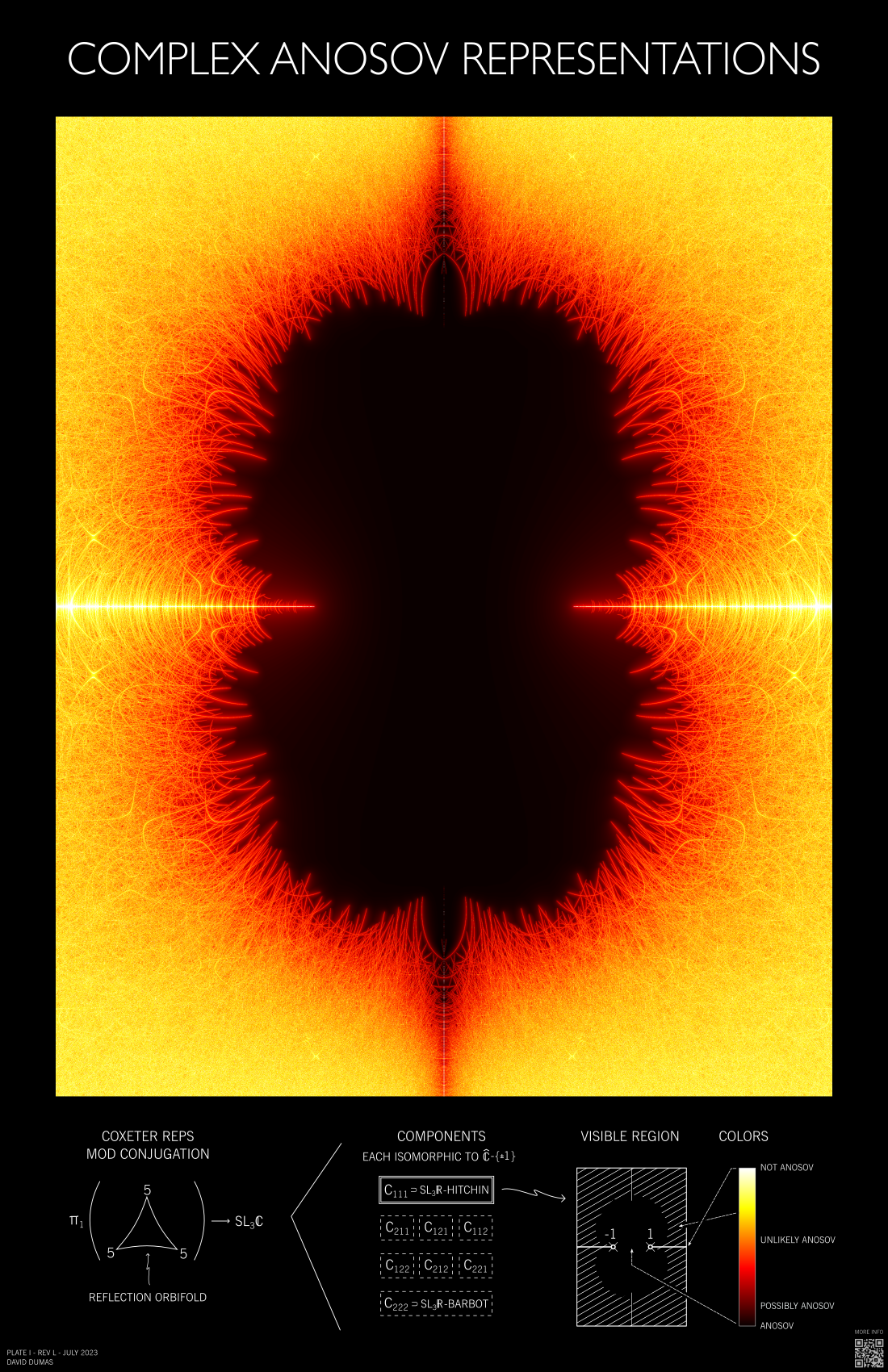
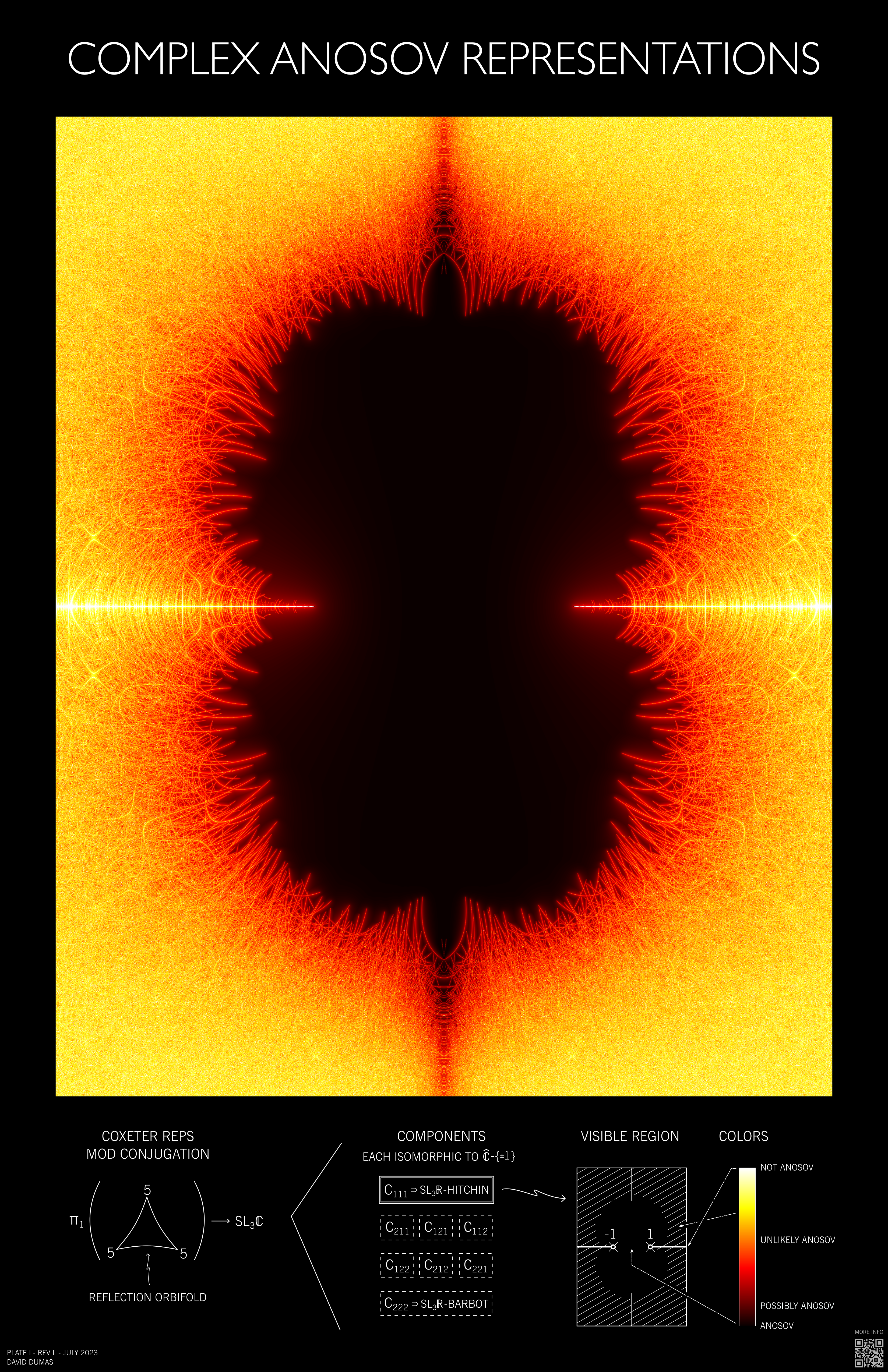
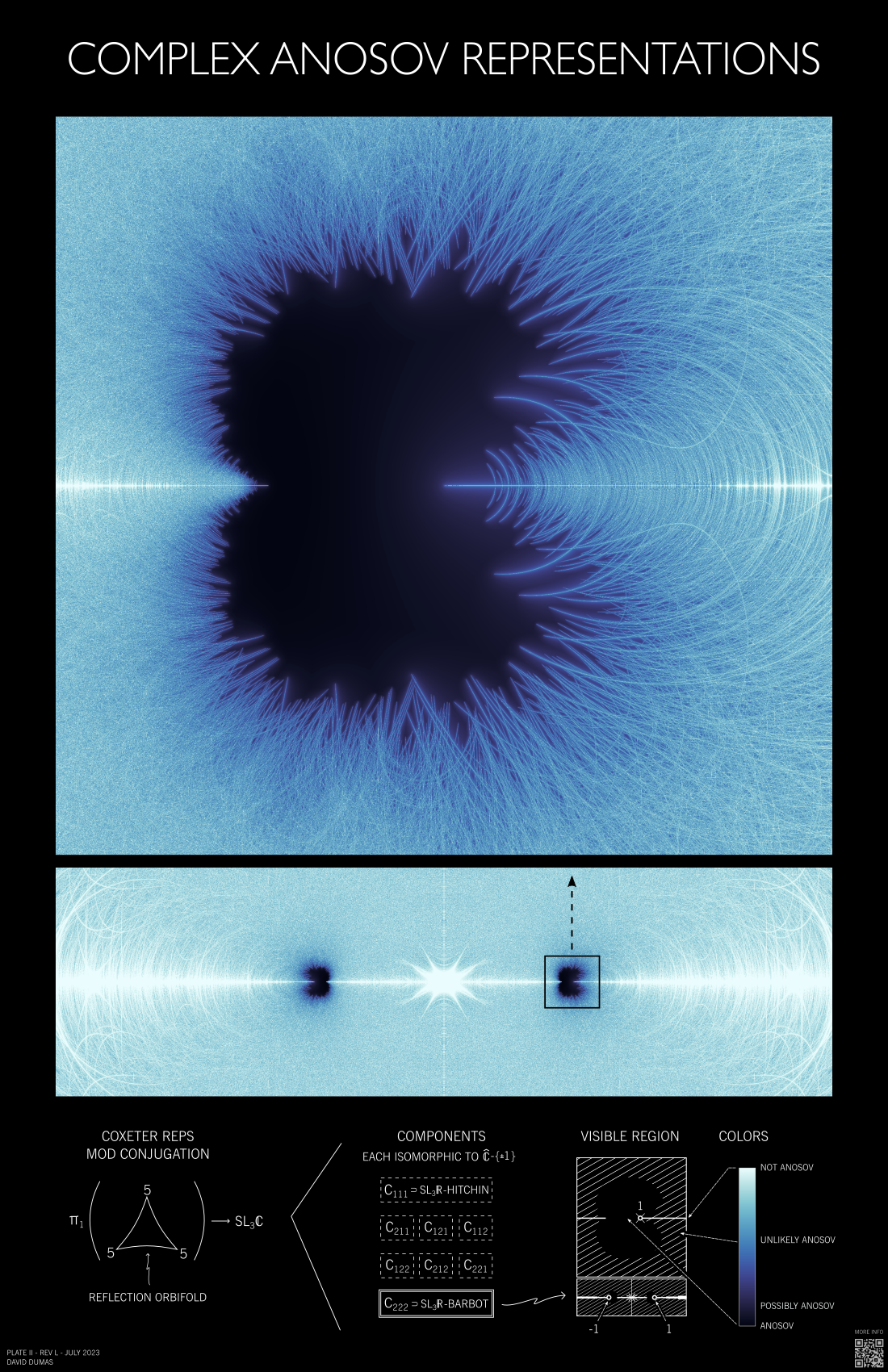
This family of homomorphisms is universal in the following sense: The set of homomorphisms $\Gamma \to \SL_3\C$ that are Coxeter (a generic condition) has 8 connected components, labeled by triples of integers $(k_1,k_2,k_3)$ with $k_i \in \{1,2\}$. Any homomorphism in component $(1,1,1)$ is conjugate to $\rho^1_s$ for a unique $s$, and similarly for component $(2,2,2)$ and $\rho^2_s$. These two components contain important classes of homomorphisms into the real form $\SL_3\R$:
We do not apply a rigorous test that classifies a representation as Anosov or not. As far as we know, criteria that apply in this generality would require infinitely many computations for each homomorphism. Instead, we use a heuristic: A collection of conditions sufficient for being non-Anosov are combined into a scalar invariant that takes on small values for most Anosov representations and is conjecturally infinite on a dense set of non-Anosov representations.
To describe this invariant, we first note that an Anosov homomorphism maps an element of $\Gamma$ of infinite order to a matrix whose eigenvalues are "well-separated", in the sense that the ratio of magnitudes of any two of them is bounded away from 1.
To quantify such separation, given an invertible $3 \times 3$ matrix $A$ let $\lambda_i(A)$ denote its eigenvalues (with multiplicity), ordered so that $|\lambda_1| \geq |\lambda_2| \geq |\lambda_3|$. For $A$ with eigenvalues of distinct magnitude, define the eigenvalue crowding of $A$ to be the positive real number $$ cr(A) = x(A) + \frac{1}{x(A)}, \; \text{ where } \; x(A) = \frac{\log |\lambda_1(A) / \lambda_2(A)|}{\log |\lambda_2(A) / \lambda_3(A) |}.$$ This function is designed so that $cr(A) \to \infty$ when the ratio of magnitudes of any pair of eigenvalues approaches 1. By construction $cr$ is constant on conjugacy classes, and it is not difficult to see that $cr(A^n) = cr(A)$ for any nonzero integer $n$. We extend the definition by setting $cr(A) = \infty$ if $A$ has a two eigenvalues of equal magnitude.
For any Anosov homomorphism $\rho : \Gamma \to \SL_3\C$, there is a uniform (finite) upper bound on the eigenvalue crowding of infinite-order elements, i.e. if we define $$\overline{cr}(\rho) := \sup \, \{ cr(\rho(\gamma)) \: | \: \gamma \in \Gamma \text{ has infinite order } \}$$ then $\overline{cr}(\rho) < \infty$ for Anosov $\rho$. Furthermore, $\overline{cr}(\rho)$ varies continuously with $\rho$ on the space of Anosov homomorphisms.
On the other hand, if a homomorphism $\rho$ maps an infinite-order element of $\Gamma$ to a matrix $A$ with $cr(A) = \infty$, then $\rho$ is not Anosov. Moreover, any limit point of a sequence of such $\rho$ is non-Anosov, since the non-Anosov set is closed.
Combining these two observations, it is reasonable to conjecture that the closure of the set $\{ \rho \: | \: \overline{cr}(\rho) = \infty \}$ is equal to the complement of the set of Anosov representations. This is analogous to the common practice of using a search for parabolic elements to visualize the quasi-Fuchsian locus in $\SL_2\C$ representation spaces (e.g. in [A], [B], [3, Chapter 10]). And there are some higher-rank results that support the use of this sort of criterion, for example in the work of Martin-Baillon on proximal stability [2].
In any case, the conjectural characterization of Anosov representations as the interior of the set where $\overline{cr}(\rho)$ is finite suggests an algorithm to visualize an approximation of that set through a finite calculation:
The resulting image should show an approximation of the Anosov set as a region of relatively dark and continuously varying colors. Outside the Anosov set, the finite supremum $\overline{cr}_E$ approximates an infinite supremum that conjecturally has value $\infty$ on a dense set. Thus we expect large values and oscillatory behavior in the non-Anosov region.
Of course this method does not certify any given representation as Anosov, but it does show certain arcs of rigorously non-Anosov representations—those where an element of $E$ is has two eigenvalues of equal magnitude, and hence $\overline{cr}_E = \infty$.
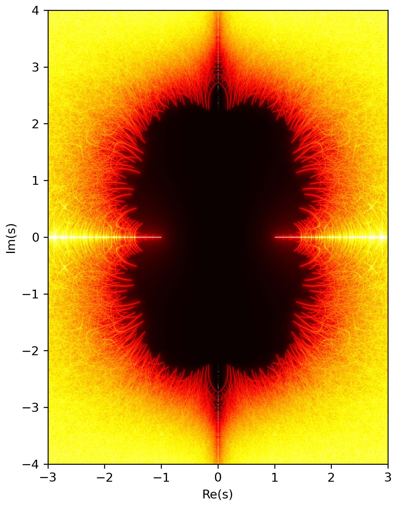
As mentioned above, the open interval $\{ \rho^1_s \: | \: s \in (-1,1) \}$ corresponds to the set of $\mathrm{SL}_3(\mathbb{R})$ Hitchin representations, while the rest of the real axis in this family consists of non-Anosov representations. As the set of Anosov representations is open and contains the Hitchin representations, it follows that the Anosov region is a neighborhood of the interval $(-1,1)$.
Poster I contains a visualization of the eigenvalue crowding function on this component. The color map ("hot" from matplotlib) varies from black to red to yellow to white, with the maximum of the range corresponding to eigenvalue crowding 200,000. As expected, the apparent complement of the Anosov set is filled with many overlapping arcs (along which two eigenvalues of an element have equal magnitude). Some of these arcs end at points where two eigenvalues values coincide, and it would be natural to ask whether any of these points are boundary points of the Anosov set.
It is also not clear whether the Anosov set in this component is connected. The picture shows many isolated dark voids among the arcs, which might represent other connected components of the Anosov set. However, experimentally it seems these voids shrink significantly as larger sets of words are used in the computation (and more arcs of equal eigenvalue magnitude appear). Whether they would disappear entirely in the limit of considering all infinite-order words is not clear.
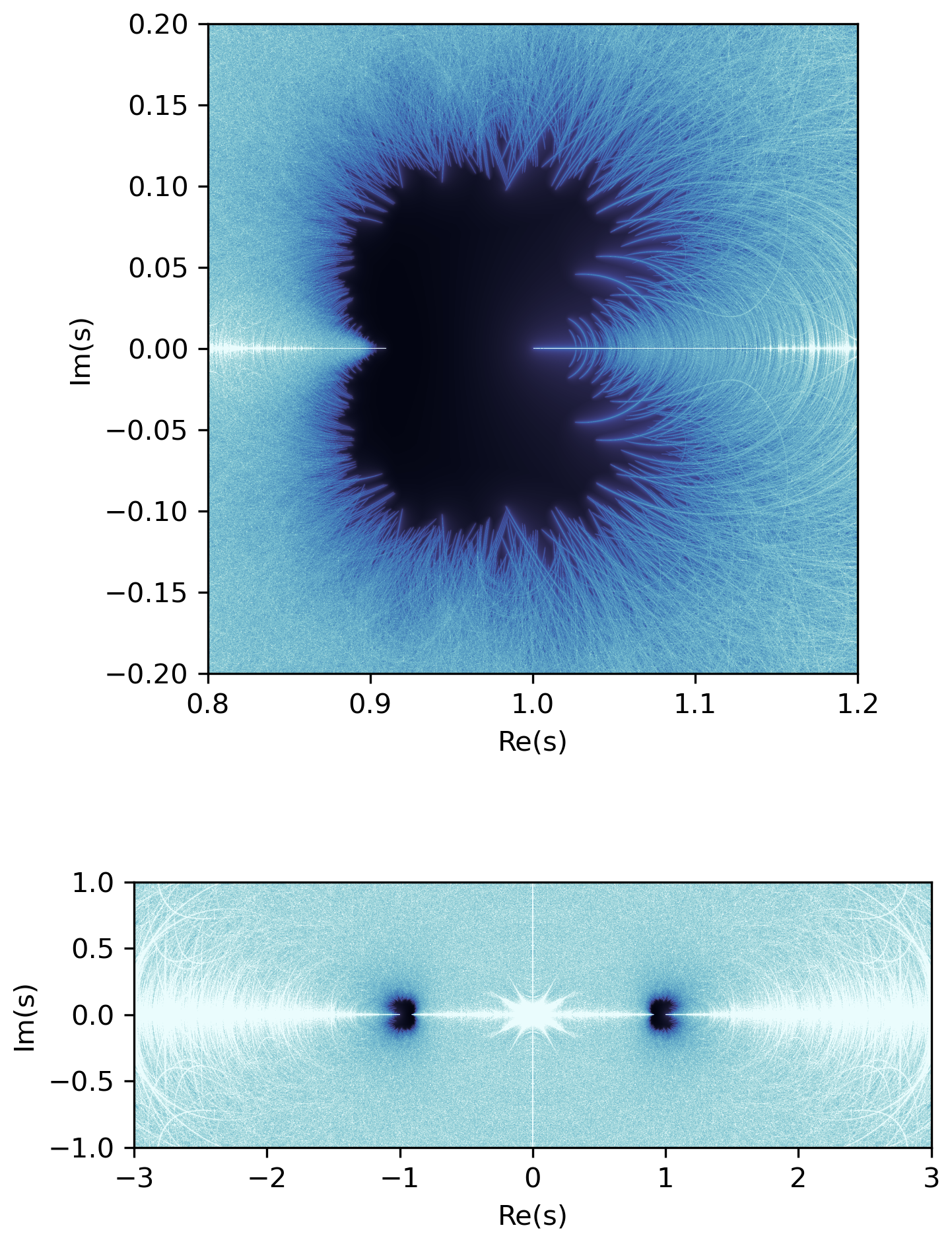
In [1], Lee, Lee, and Stecker show that the part of the family on the real line $\{ \rho^2_s \: | \: s \in \R \setminus \{-1,1\} \}$ intersects the Anosov set in two intervals: $(-1,-\kappa)$ and $(\kappa,1)$ for some $\kappa \in (0,1)$ (explicitly computable using their methods).
Poster II contains a visualization of the eigenvalue crowding function on this component. Real values of $s$ lie along the horizontal line through the center of each image on the poster. The color map ("ice" from cmocean) varies from black to blue to white, with the maximum of the range corresponding to eigenvalue crowding 200,000. The Anosov regions are quite small relative to the size of the interval $(-1,1)$, so the poster contains both a wide view and a detail view centered on one of the real Anosov intervals.
In this case, representations on the imaginary axis are not Anosov (as they take values in a compact subgroup of $\SL_3\C$), so the two intervals of real Anosov representations lie in distinct components of the complex Anosov set. Analogously to the Hitchin case, it is not clear if there are other complex Anosov components.
As explained above, there are two main steps:
The enumeration step is a preliminary calculation that can be re-used by each raster calculation. It proceeds by considering words of length less than a configurable threshold and selecting a subset that provides a representative of each conjugacy class of infinite-order elements thus obtained. Increasing the length threshold gives larger collections of words and thus more detailed pictures, at the cost of a more expensive computation in both the enumeration and raster calculation steps.
Initial images for this project were created using a word list generated by a simple Python program that used the Coxeter group structure to select conjugacy class representatives. This allowed a word length limit of 21 before becoming memory-limited. The final images used a larger word list generated by Florian Stecker (using a more efficient C program), which included words of length up to 24.
This trivially parallelizable task (one calculation per mesh point, all independent of one another) was handled by a pool of Python programs working parallel and drawing tasks from a shared queue into which data about each of the mesh points was inserted. Each component has reflection symmetry to the Anosov set and the crowding function in both $x$ and $y$ axes, allowing the number of grid points to be reduced by a factor of 2 or 4 depending on the region of interest.
Most of the final calculations were performed on 24-core machines in the SABER cluster at the University of Illinois at Chicago. The final raster computations for the posters required about 7200 CPU-hours, with about the same amount of computer time used in earlier exploratory calculations. Eigenvalue crowding data were stored as 2-dimensional arrays of floats in HDF5 data files, and later converted to a bitmap image by a separate Python program developed for post-processing.The typeface and layout of the lower section of each poster is loosely modeled after the design of Apollo-era NASA technical documentation (e.g. figures in the LM Orientation Training Course from April 1966).
The posters were created with Inkscape.
It would be natural to explore Anosov representations in the other components of the set of Coxeter representations. Our approach used the invariance of the $(1,1,1)$ and $(2,2,2)$ components under the outer automorphism group of $\Gamma$ in the word enumeration step, so further work in this direction would require changes to that preliminary calculation.
Also, the raster computation step would seem to naturally lend itself to GPU-based computing. This might offer enough of a speed improvement to allow nearly real-time generation of these images.
This material is based upon work supported by the National Science Foundation. Any opinions, findings, and conclusions or recommendations expressed in this material are those of the author and do not necessarily reflect the views of the National Science Foundation.

