Lecture 18
Comparison sorts
MCS 275 Spring 2021
Emily Dumas
Lecture 18: Comparison sorts
Course bulletins:
- Quiz 6 due Noon CST Tuesday.
- Project 2 due 6pm CST Friday. Autograder open.
- Worksheet 7 coming soon.
Growth rates
Let's look at the functions $n$, $n \log(n)$, and $n^2$ as $n$ grows.
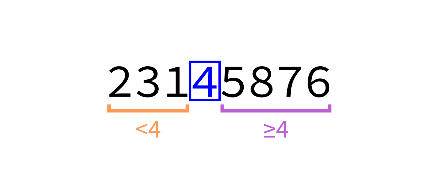
Partition
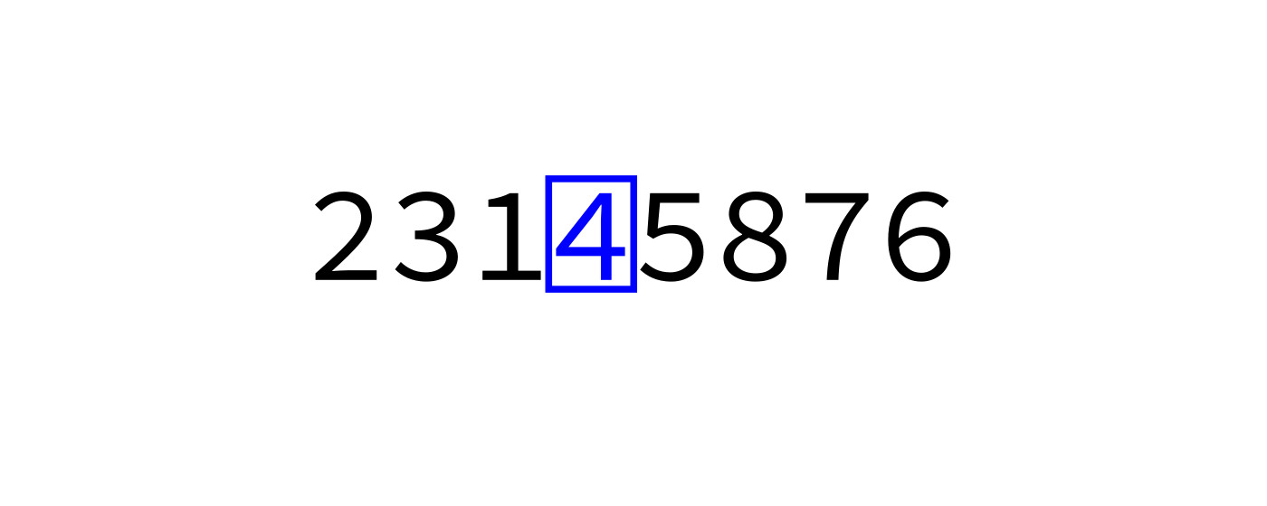
We say L is partitioned if there is an element (the pivot) so that:
- The pivot is in its final sorted position
- Any element less than the pivot appears before it
- Any element greater than or equal to the pivot appears after it
partition(L,start,end) should move around elements of L between indices start and end to achieve this,
returning the pivot position.
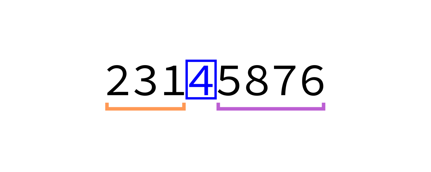
quicksort:
Input: list L and indices start and end.
Goal: reorder elements of L so that L[start:end] is sorted.
- If
(end-start)is less than or equal to 1, return immediately. - Otherwise, call
partition(L,start,end)to partition the list, lettingmbe the final location of the pivot. - Call
quicksort(L,start,m)andquicksort(L,m+1,end)to sort the parts of the list on either side of the pivot.
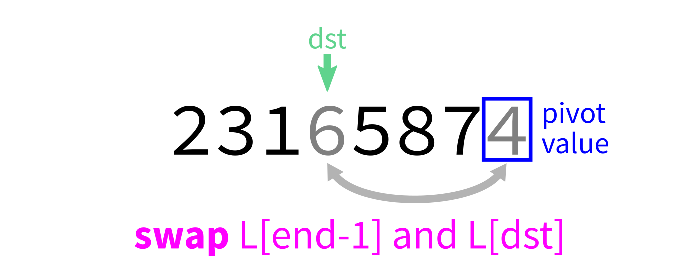
Partition algorithm
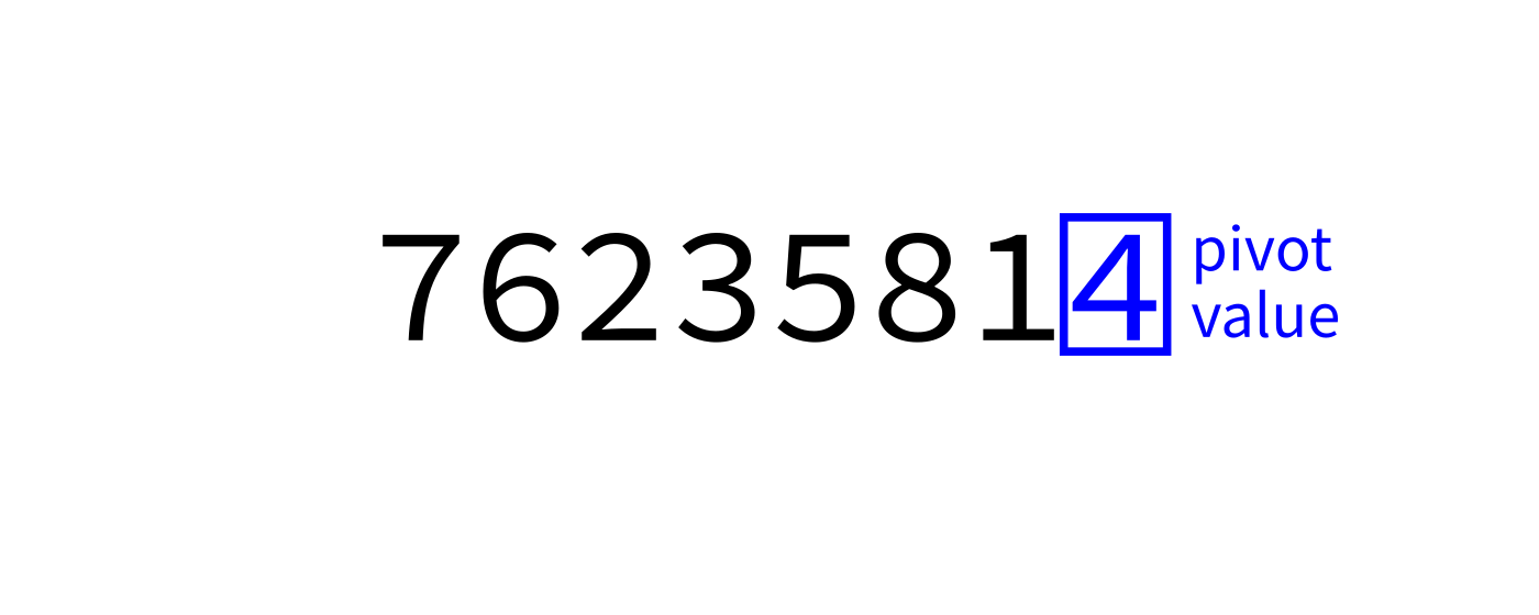
We will always use L[end-1] as the pivot (though there are other common choices).
There is an algorithm for partition based on the idea of using swaps to move all small elements to a contiguous block at the beginning.
It makes a single pass through the entire list.
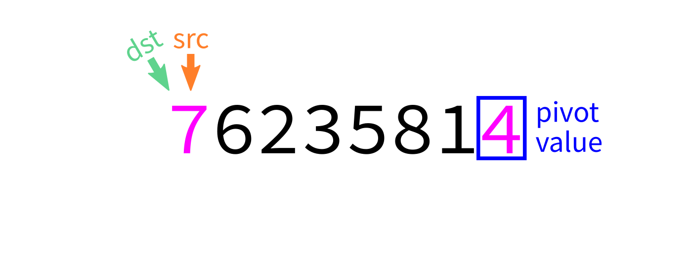
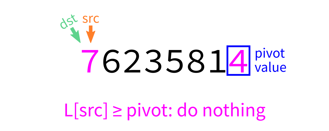
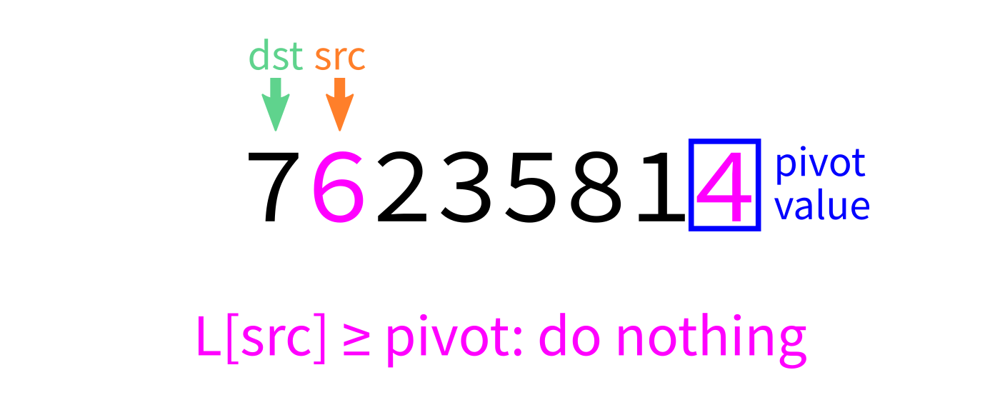
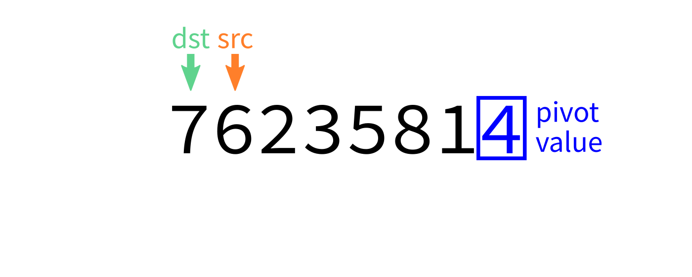
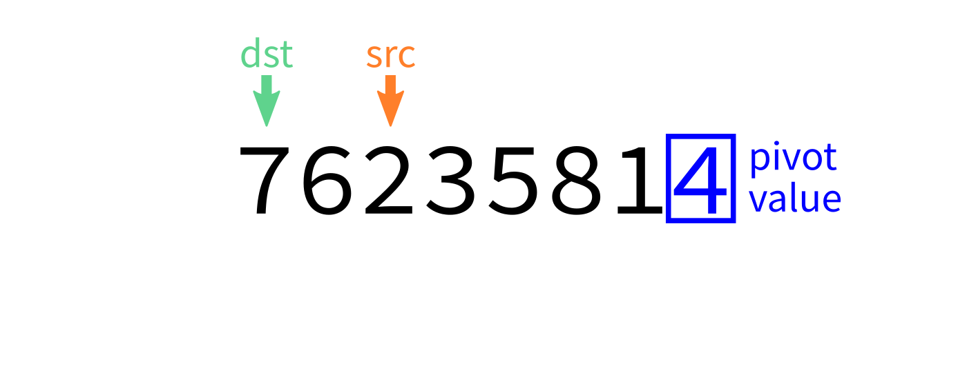
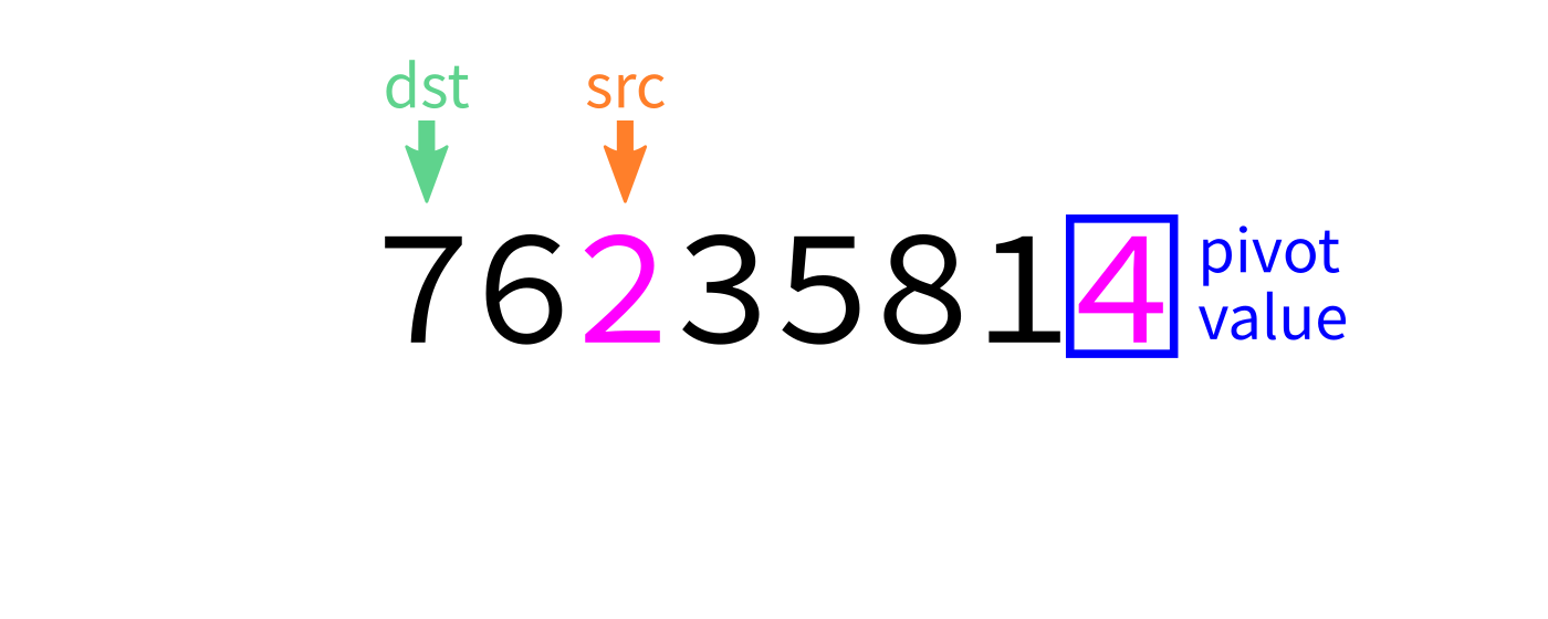
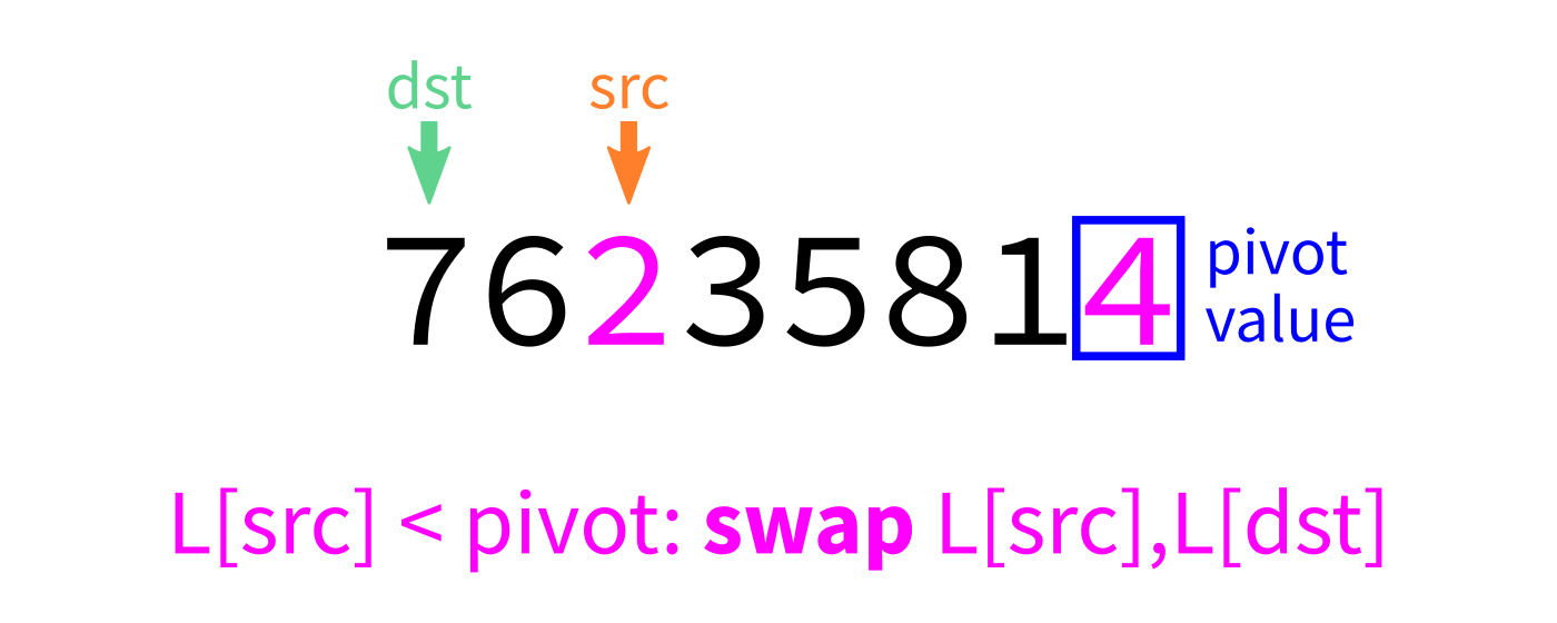
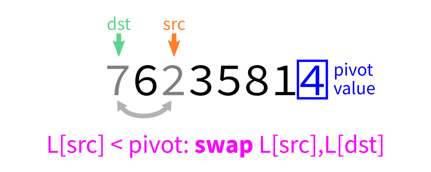
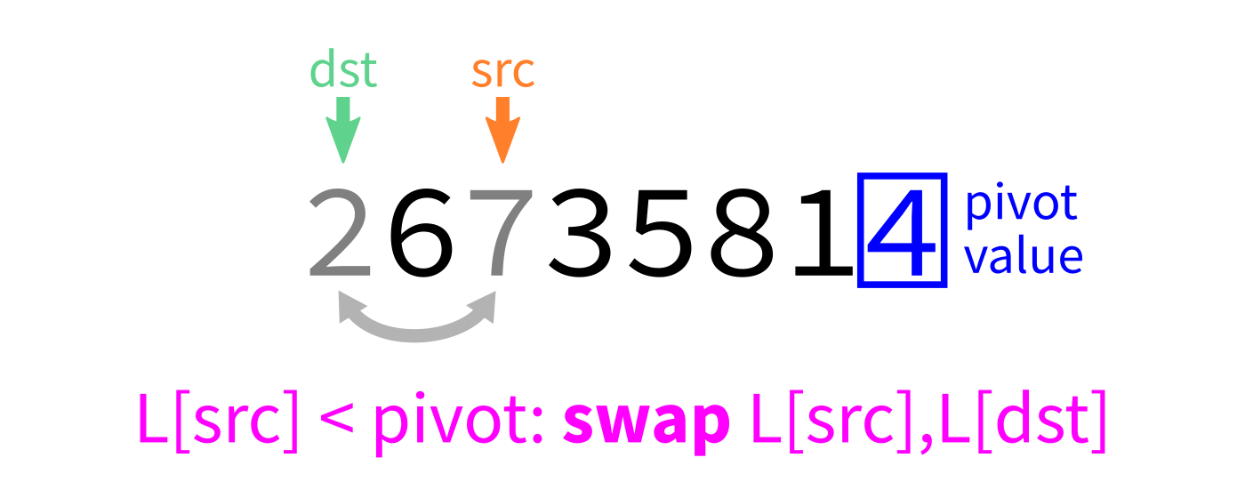
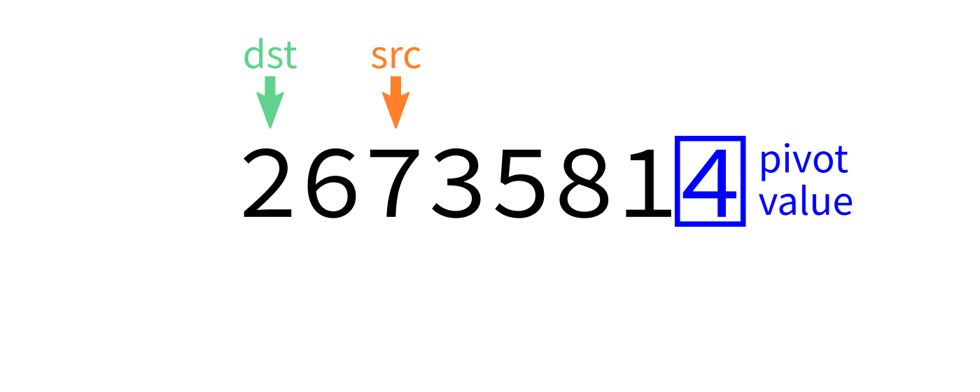
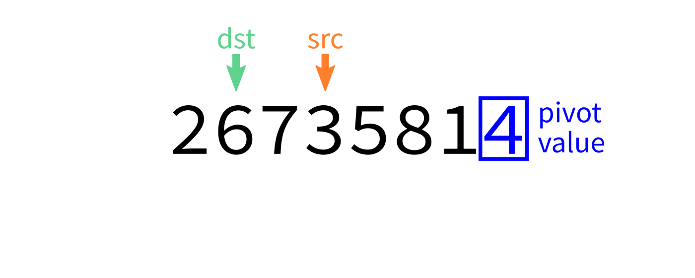
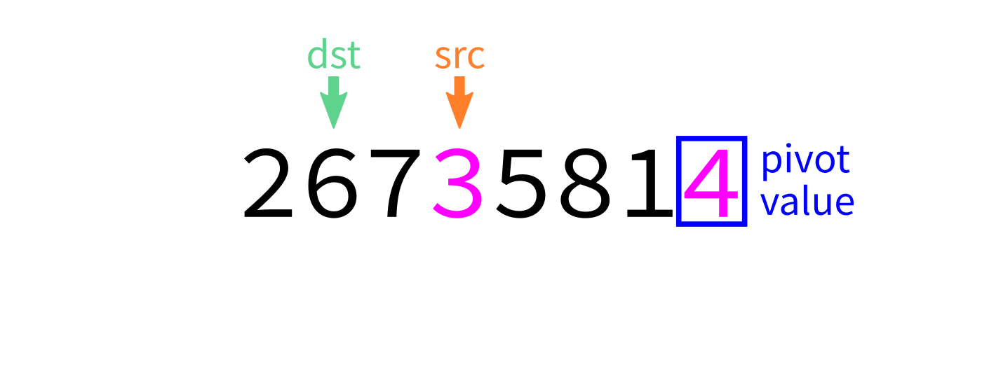
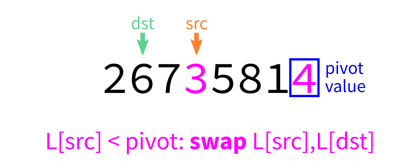
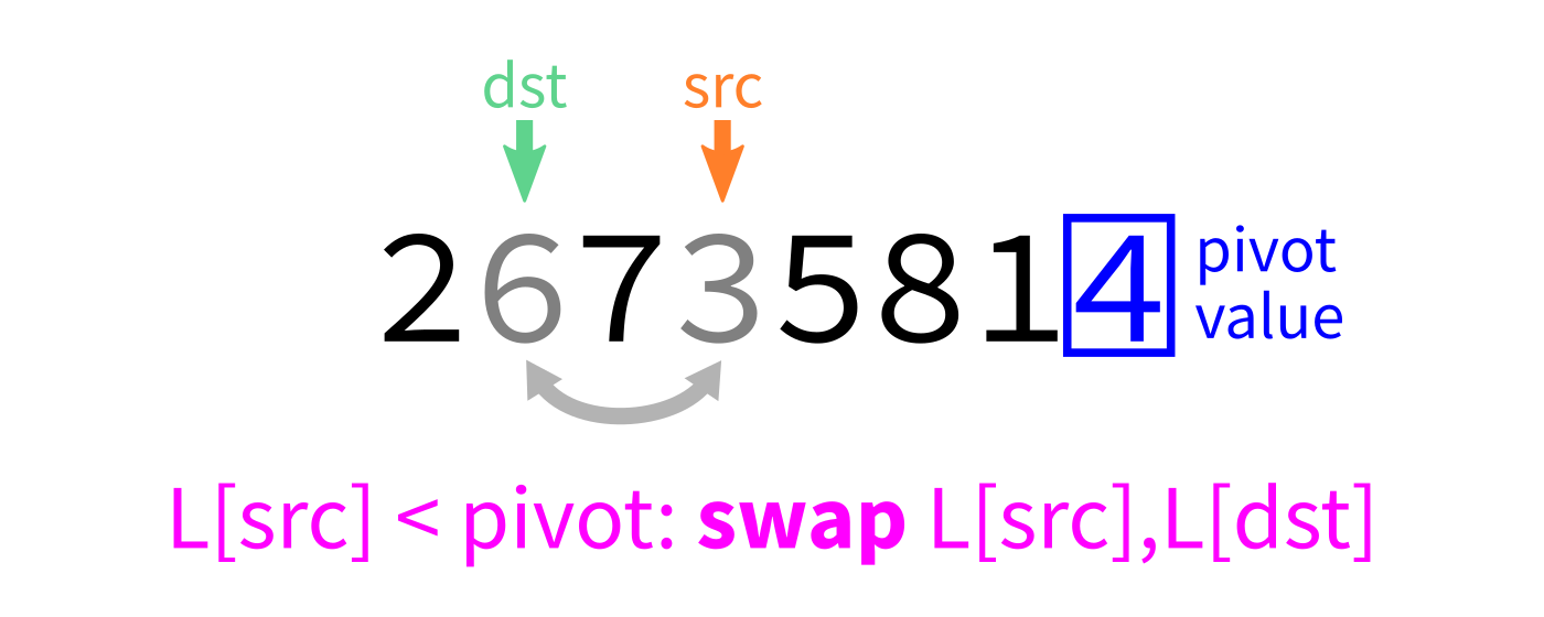
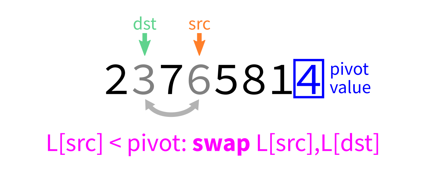
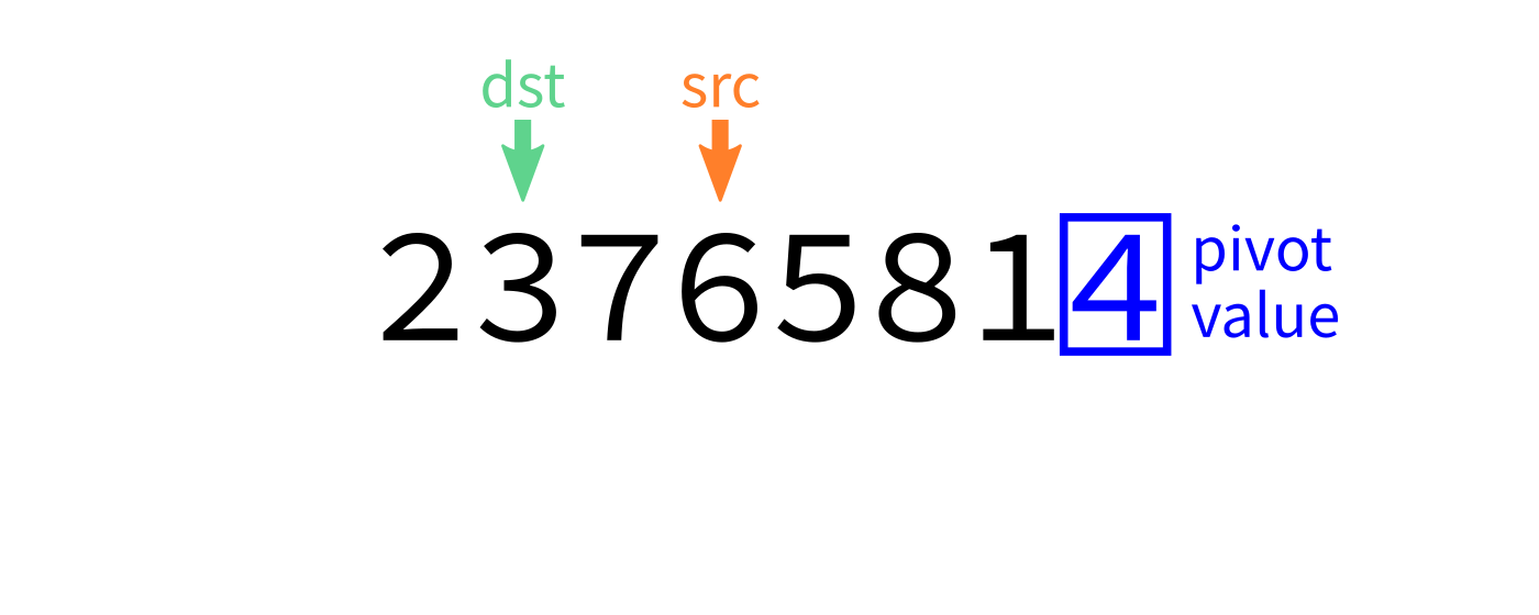
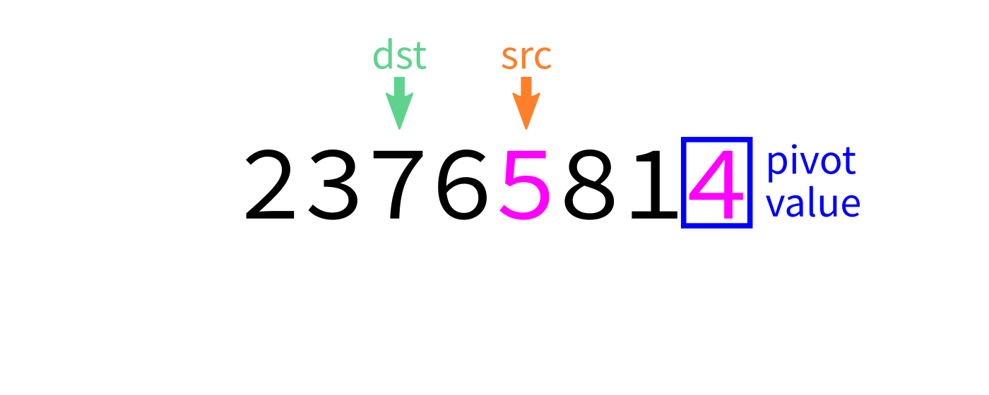
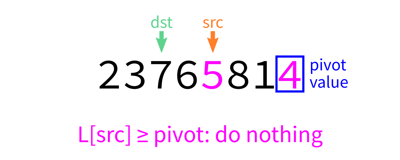
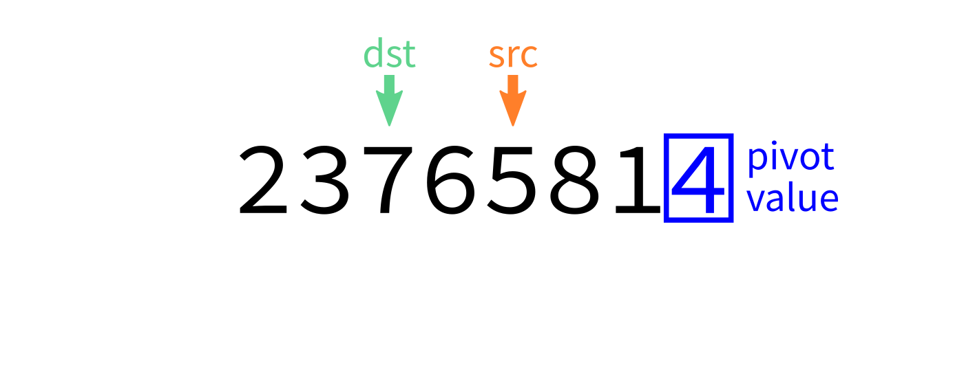
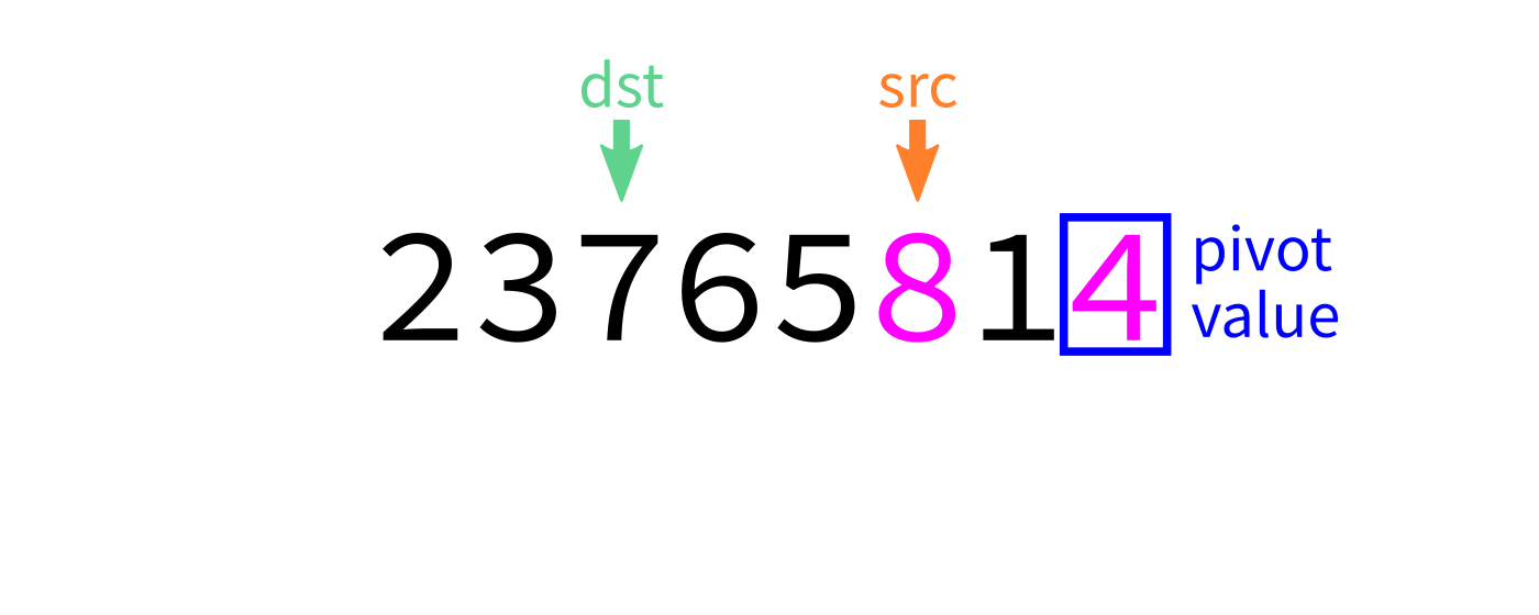
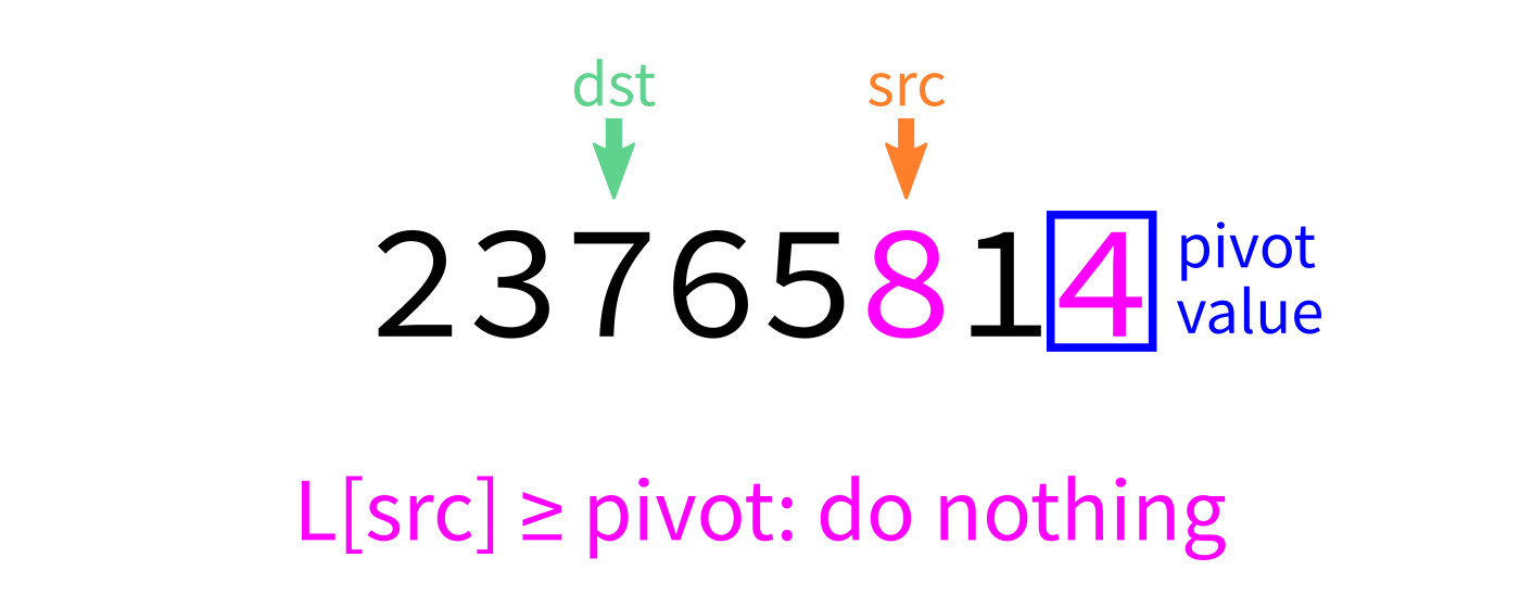
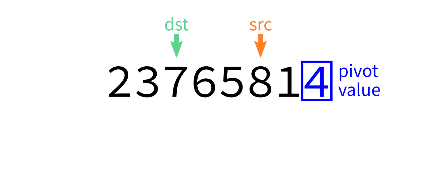
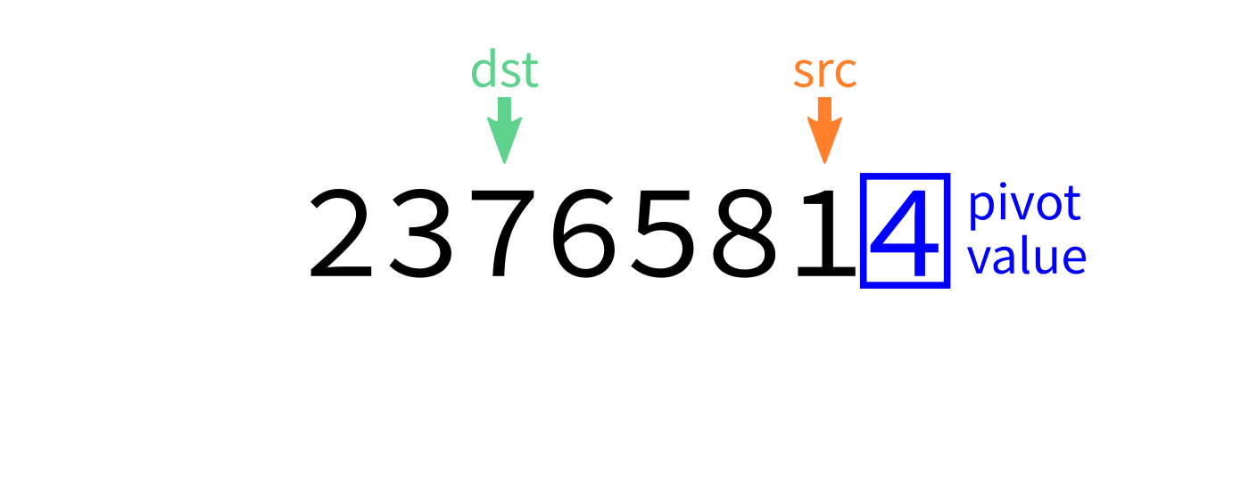
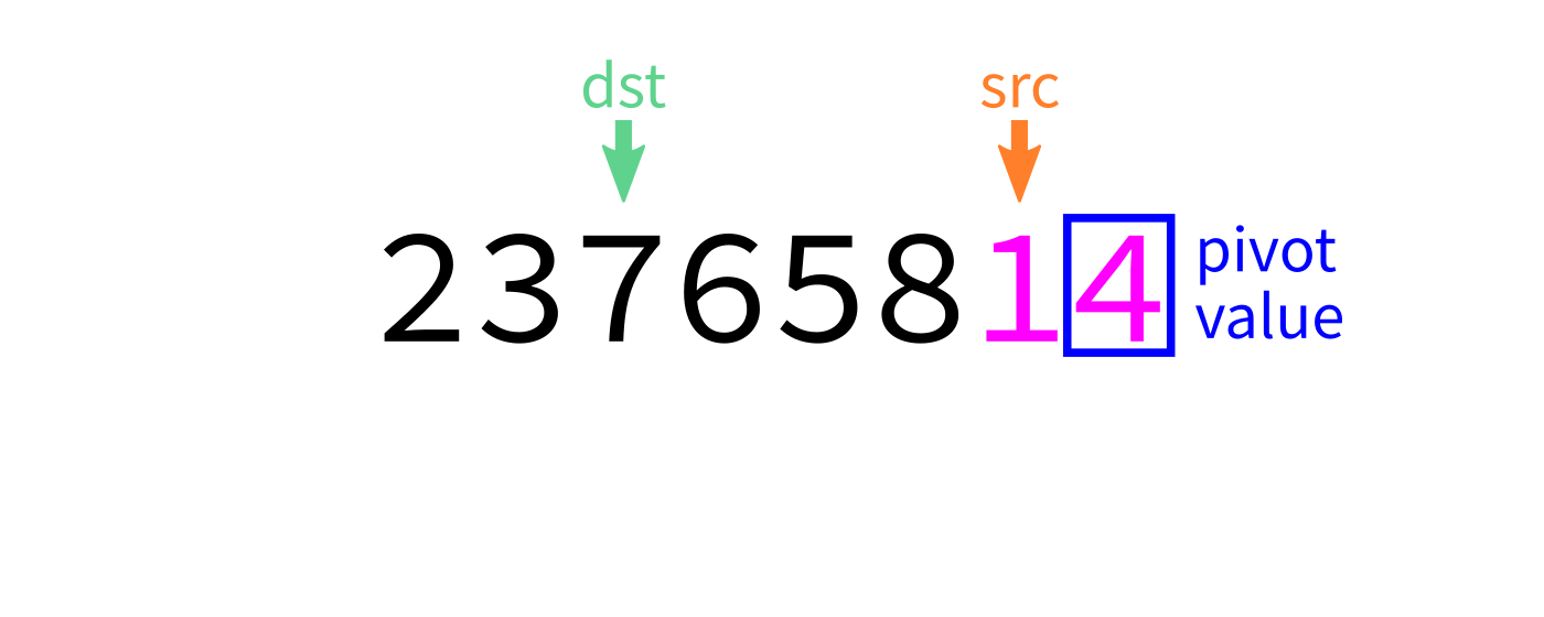
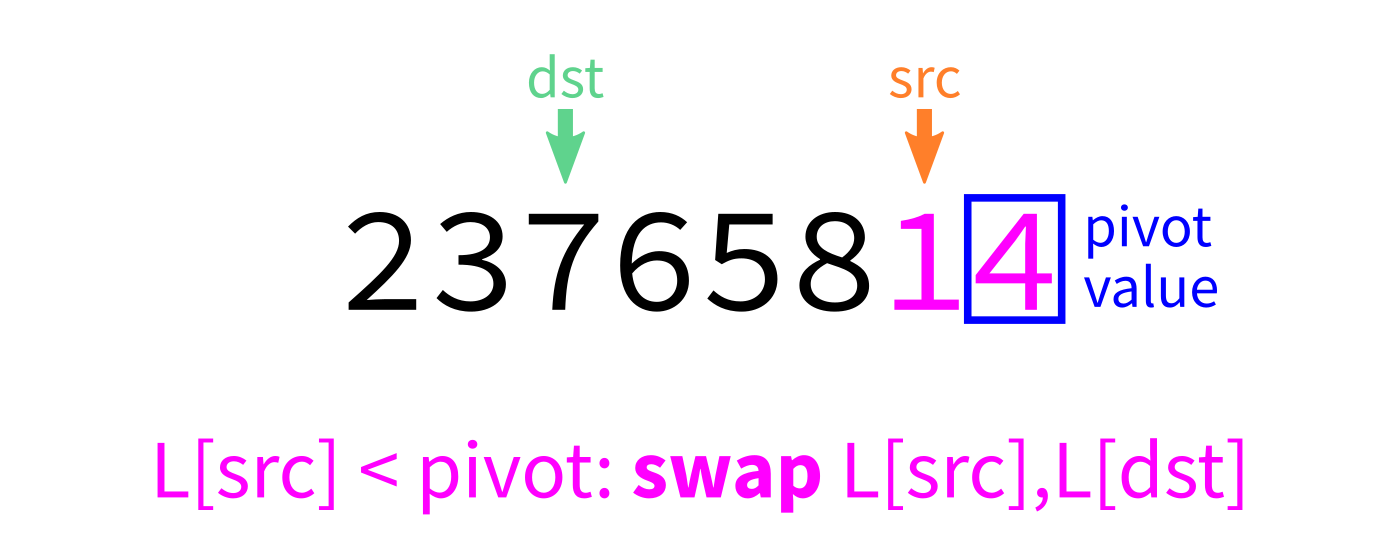
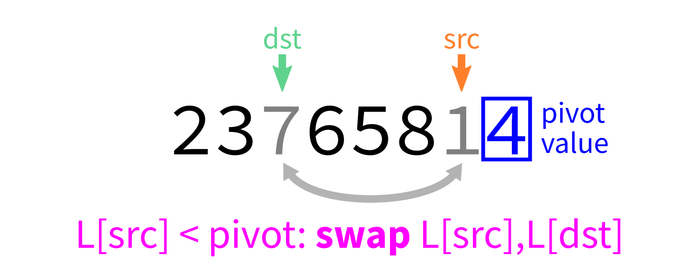
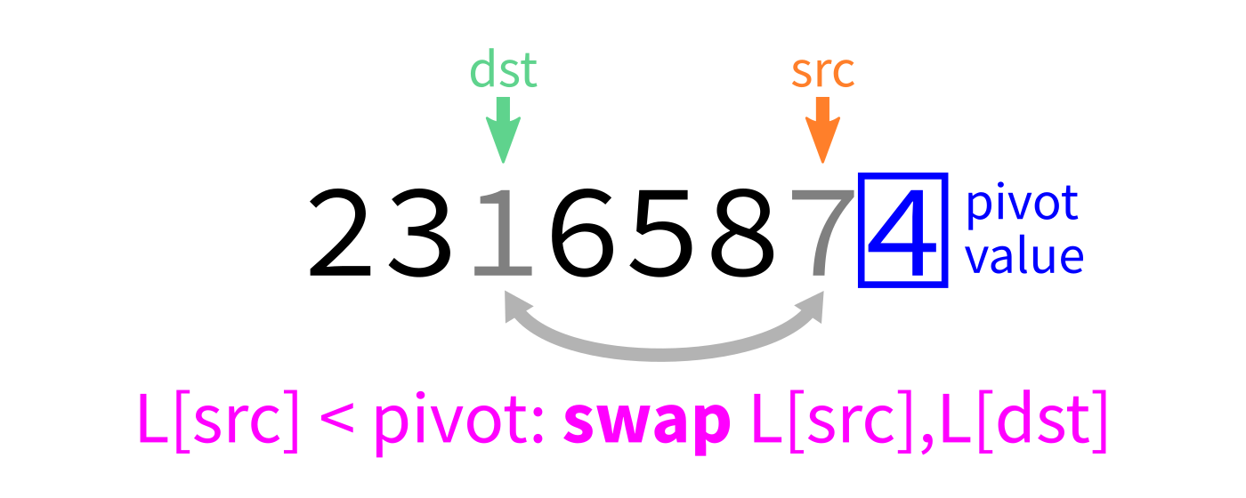
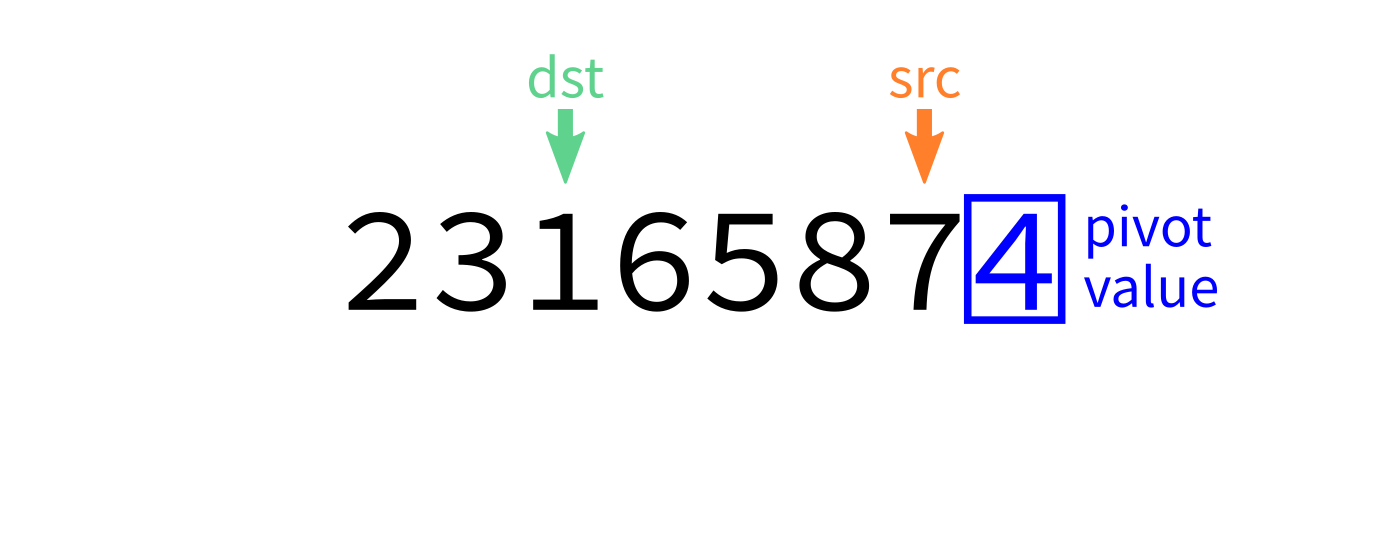
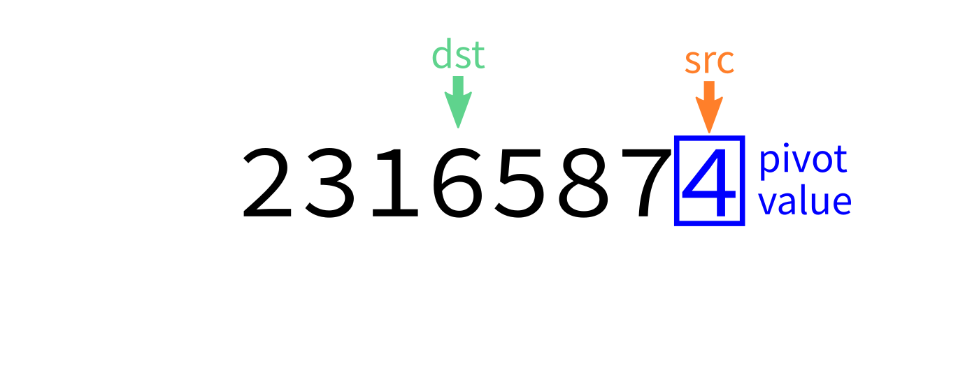
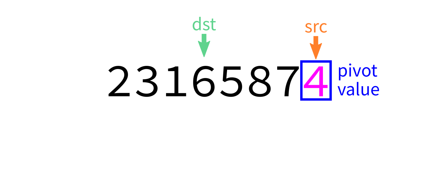
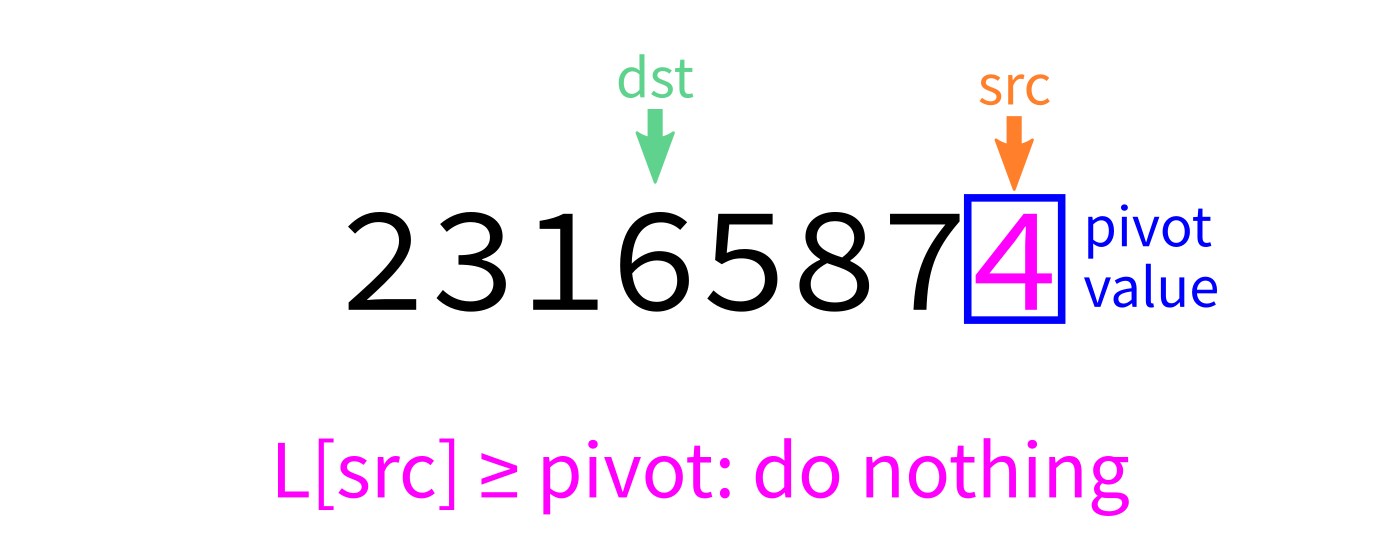
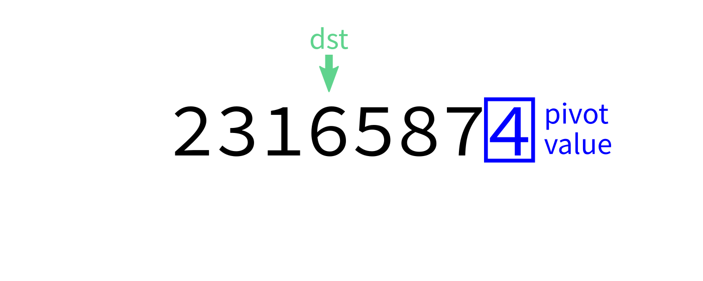
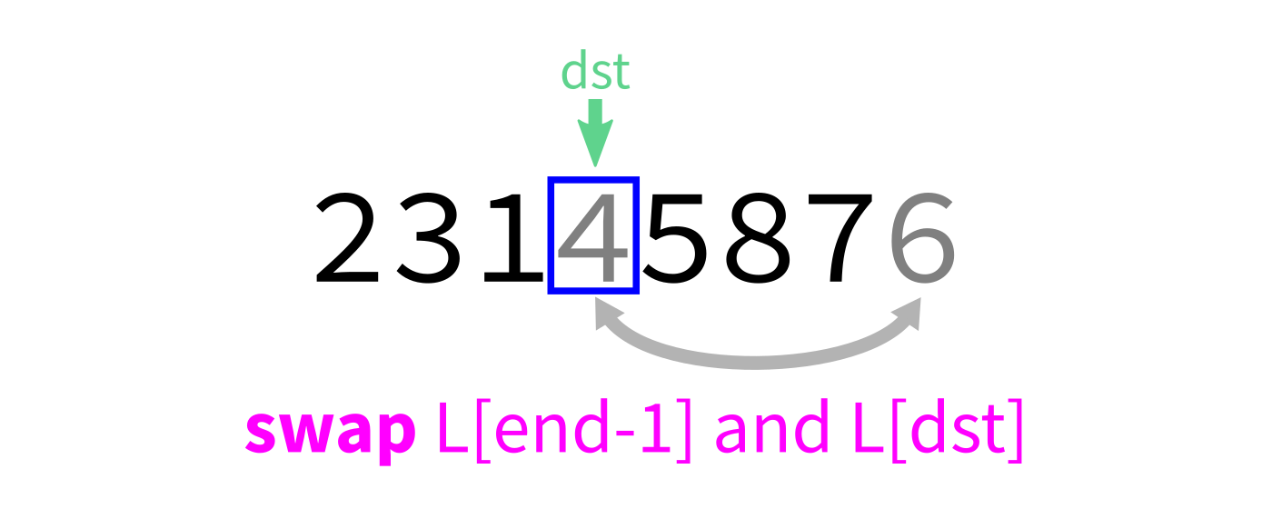
Partition visualization


Coding time
Let's implement partition (with last element pivot) in Python.
partition:
Input: list L and indices start and end.
Goal: Take L[end-1] as a pivot, and reorder elements of L to partition L[start:end] accordingly.
- Let
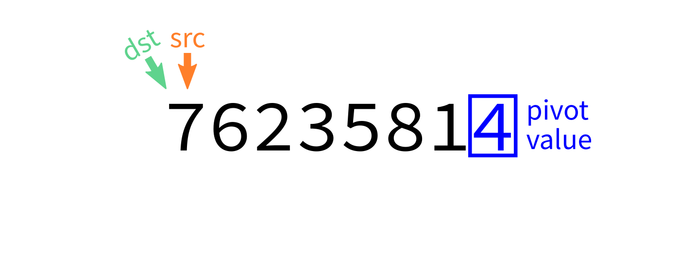
pivot=L[end-1]. - Initialize integer index
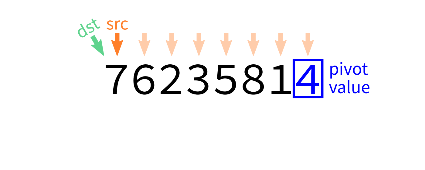
dst=start. - For each integer
srcfromstarttoend-1: - If
L[src] < pivot, swapL[src]andL[dst]. - Increase
dstby 1. - Swap
L[end-1]andL[dst]to put the pivot in its proper place. - Return
dst.
Other partition strategories
Popular choices for the pivot:
- The last element,
L[end-1](used in lecture today) - The first element,
L[start] - A random element of
L[start:end] - The element
L[(start+end)//2] - An element near the median of
L[start:end](more complicated to find!)
How to choose?
Knowing something about your starting data may guide choice of partition strategy (or even the choice to use something other than quicksort).
Almost-sorted data is a common special case where first or last pivots are bad.
Efficiency
Theorem: If you measure the time cost of quicksort in any of these terms
- Number of comparisons made
- Number of swaps or assignments
- Number of Python statements executed
then the cost to sort a list of length $n$ is less than $C n^2$, for some constant $C$.
But if you average over all possible orders of the input data, the result is less than $C n \log(n)$.
Bad case
What if we ask our version of quicksort to sort a list that is already sorted?
Recursion depth is $n$ (whereas if the pivot is always the median it would be $\approx \log_2 n$).
Number of comparisons $\approx C n^2$. Very slow!
Stability
A sort is called stable if items that compare as equal stay in the same relative order after sorting.
This could be important if the items are more complex objects we want to sort by one attribute (e.g. sort alphabetized employee records by hiring year).
As we implemented them:
- Mergesort is stable
- Quicksort is not stable
Efficiency summary
| Algorithm | Time (worst) | Time (average) | Stable? | Space |
|---|---|---|---|---|
| Mergesort | $C n \log(n)$ | $C n\log(n)$ | Yes | $C n$ |
| Quicksort | $C n^2$ | $C n\log(n)$ | No | $C$ |
(Every time $C$ is used, it represents a different constant.)
Other comparison sorts
- Insertion sort -- Convert the beginning of the list to a sorted list, starting with one element and growing by one element at a time.
- Bubble sort -- Process the list from left to right. Any time two adjacent elements are in the wrong order, switch them. Repeat $n$ times.
Efficiency summary
| Algorithm | Time (worst) | Time (average) | Stable? | Space |
|---|---|---|---|---|
| Mergesort | $C n \log(n)$ | $C n\log(n)$ | Yes | $C n$ |
| Quicksort | $C n^2$ | $C n\log(n)$ | No | $C$ |
| Insertion | $C n^2$ | $C n^2$ | Yes | $C$ |
| Bubble | $C n^2$ | $C n^2$ | Yes | $C$ |
(Every time $C$ is used, it represents a different constant.)
Closing thoughts on sorting
Mergesort is rarely a bad choice. It is stable and sorts in $C n \log(n)$ time. Nearly sorted input is not a pathological case. Its main weakness is its use of memory proportional to the input size.
Heapsort, which we'll discuss later, has $C n \log(n)$ running time and uses constant space, but it is not stable.
There are stable comparison sorts with $C n \log(n)$ running time and constant space (best in every category!) though they are more complex.
If swaps and comparisons have very different cost, it may be important to select an algorithm that minimizes one of them. Python's list.sort assumes that comparisons are expensive, and uses Timsort.
Quadratic danger
Algorithms that take time proportional to $n^2$ are a big source of real-world trouble. They are often fast enough in small-scale tests to not be noticed as a problem, yet are slow enough for large inputs to disable the fastest computers.
References
Unchanged from Lecture 17
- You can refer to the general references about recursion that have appeared in several recent lectures. The rest of this list is specific to mergesort and quicksort.
- Making nice visualizations of sorting algorithms is a cottage industry in CS education. Some you might like to check out:
- 2D visualization through color sorting by Linus Lee
- Animated bar graph visualization of many sorting algorithms by Alex Macy
- Slanted line animated visualizations of mergesort and quicksort by Mike Bostock
Revision history
- 2021-02-22 Fixed partition visualization
- 2021-02-22 Initial publication